Data Types¶

Many parameters across ARD can be configured in different modes depending on your data and accuracy requirements. This page explains each data type and how to use them.

Overview¶

When a parameter supports multiple data types, you'll see mode selector tabs at the top of the field:

Tab Label	Data Type	Description
Value	Numeric	A single constant number with a unit
1D Map	Map1D	A 2D lookup table (one input → one output)
2D Map	Map2D	A 3D lookup table (two inputs → one output)
Expression	Expression	A mathematical formula with variables

Not all parameters support every mode. The available tabs depend on the specific parameter — for example, tyre radii support Value, 2D Map, and Expression, while spring rates may support Value and 1D Map.

Value (Numeric)¶

Value Mode

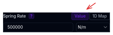
The simplest mode. Enter a single number with a unit.

UI Layout: - Left: Numeric input field - Right: Unit dropdown selector

When to use: - You have a single known value - The parameter doesn't change with operating conditions - Starting a new setup and want simplicity - This is the recommended default for most parameters

Example: - Loaded radius: 0.285 m - Tyre rate: 200000 N/m - Inertia: 0.8 kgm²

1D Map (Map1D)¶

1D Map Mode

A lookup table that maps one input variable to one output value. Displayed as a line chart.

UI Layout: - Closed: Mini line plot thumbnail (clickable to expand) - Open (Dialog): - Left: Spreadsheet with two columns (X input, Y output) - Right: Live line chart updating in real-time

1D Map UI

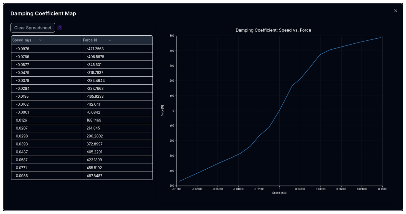
Structure: - X-axis: Input variable (e.g., wheel travel, speed) - Y-axis: Output value (e.g., spring rate, damping force)

Example — Spring rate vs displacement:

Displacement (mm)	Spring Rate (N/mm)
0	80
10	85
20	95
30	120
40	180

When to use: - Parameter varies with one operating condition - You have test data relating input to output - Non-linear behaviour needs to be captured (e.g., progressive springs)

Requirements: - X-axis values must be strictly monotonically increasing (each value larger than the previous) - The platform highlights rows in red if X-axis ordering is violated - An auto-sort button is available to fix ordering

Spreadsheet Features: - Right-click context menu for adding/deleting rows - Keyboard shortcuts: Ctrl+C/V (copy/paste), Ctrl+Z (undo), Delete (clear cell) - Paste data directly from Excel or Google Sheets

2D Map (Map2D)¶

2D Map Mode

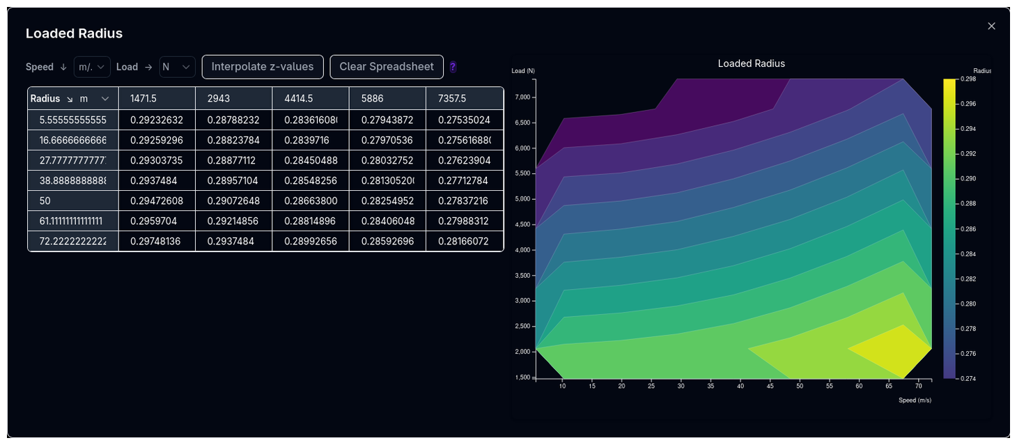
A lookup table that maps two input variables to one output value. Displayed as a heatmap/contour plot.

UI Layout: - Closed: Mini heatmap thumbnail (clickable to expand) - Open (Dialog): - Left: Spreadsheet with X-axis (columns), Y-axis (rows), and Z-values (cells) - Right: Live heatmap/contour visualization with colour legend

2D Map UI Structure: - X-axis: First input variable (e.g., speed) - Y-axis: Second input variable (e.g., vertical load) - Z-values: Output value at each (X, Y) combination (e.g., loaded radius)

Example — Loaded radius vs speed and load:

Load (N) ↓ \ Speed (m/s) →	0	20	40	60
1500	0.282	0.283	0.284	0.285
2500	0.275	0.276	0.277	0.278
3500	0.268	0.269	0.270	0.271

When to use: - Parameter varies with two operating conditions simultaneously - You have comprehensive test data (e.g., from tyre testing rigs) - High-fidelity modelling where single-variable dependency is insufficient

Requirements: - Both X and Y axis values should be monotonically increasing - Map must cover the full expected operating range of the simulation - Outside the map range, the platform extrapolates — ensure boundaries are realistic

Spreadsheet Features: - Right-click context menu for adding/deleting rows and columns - Keyboard shortcuts: Ctrl+C/V (copy/paste), Ctrl+Z (undo), Delete (clear cell) - Paste data directly from Excel or Google Sheets

Expression¶

Expression Mode

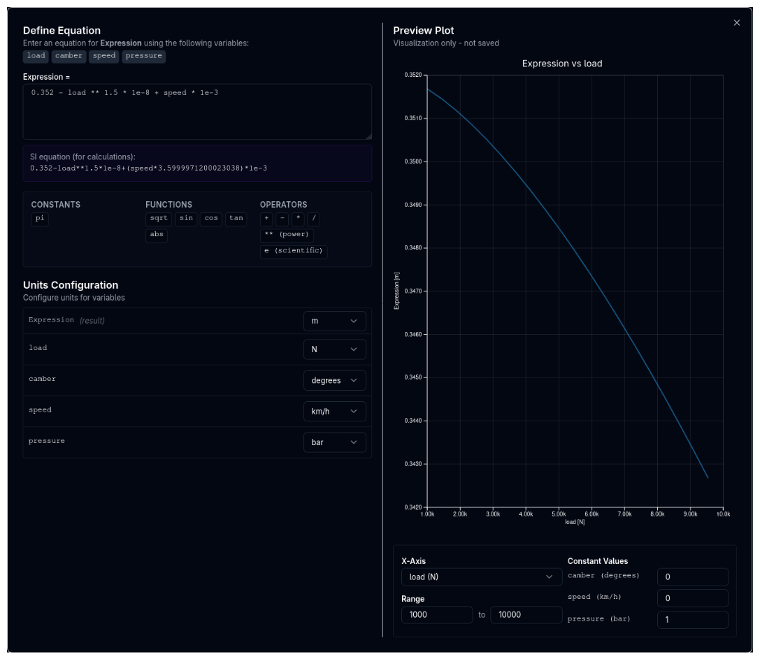
A mathematical formula evaluated at each simulation step. The most flexible mode.

UI Layout: - Closed: "Edit Equation" button - Open (Dialog): - Left: Expression editor with: - Text input area for the equation - Available variables shown as tags - Reference guide (constants, functions, operators) - Unit configuration table for each variable - Real-time validation with error messages - Right: Live plot preview of the expression

Expression Mode UI How it works: You write a single mathematical expression that computes the result. The expression is a single, fully expanded formula — no intermediate variable assignments.

Available Operators and Functions:

Type	Available
Operators	`+`, `-`, ``, `/`, `*` (power), `e` (scientific notation)
Functions	`sqrt()`, `sin()`, `cos()`, `tan()`, `abs()`
Constants	`pi`

Available Variables: The variables depend on the specific parameter. Common variables include:

load — Vertical load
speed — Vehicle speed
camber — Camber angle
pressure — Inflation pressure

Each variable has a configurable unit. The platform automatically converts the expression coefficients to match your selected units.

Example — Loaded radius with load dependency:

0.285 - load / 200000

Example — Rolling radius with speed growth:

(0.285 - load / 200000) * 1.03 + speed * 0.0001

Example — Radius with pressure correction:

0.285 - load / 200000 + (pressure - 180000) * 1e-6

When to use: - You have a theoretical or empirical relationship - Need more flexibility than a lookup table - Custom models or research applications - The relationship follows a known formula

Validation: - Parentheses must be balanced - Only allowed variables, functions, and constants can be used - Maximum length: 500 characters - ^ is automatically converted to **

Display Formatting: The editor formats expressions for readability: - **2 displays as superscript ² - * displays as × - / displays as ÷ - sqrt( displays as √(

Single Expression Only

The expression must be a single, fully expanded formula. You cannot define intermediate variables or use multi-line expressions. For example, write 0.285 - load / 200000 + (pressure - 180000) * 1e-6 rather than assigning intermediate results.

Choosing the Right Data Type¶

graph TD
    Q1{Do you have<br/>measured data?}
    Q1 -->|No| V[Use Value]
    Q1 -->|Yes| Q2{How many<br/>input variables?}
    Q2 -->|None - single value| V
    Q2 -->|One variable| M1[Use 1D Map]
    Q2 -->|Two variables| M2[Use 2D Map]
    Q1 -->|I have a formula| E[Use Expression]

    style V fill:#10b981,color:#fff
    style M1 fill:#6366f1,color:#fff
    style M2 fill:#8b5cf6,color:#fff
    style E fill:#f59e0b,color:#fff

Scenario	Recommended
Single known value (e.g., tyre radius from spec sheet)	Value
Data varies with one input (e.g., spring rate vs displacement)	1D Map
Data varies with two inputs (e.g., radius vs speed and load)	2D Map
Known formula or empirical relationship	Expression
No data available, starting fresh	Value (simplest)

Edit Tracking¶

All data types support edit tracking. When you modify a value, the field highlights in yellow to indicate unsaved changes. This applies to:

Numeric inputs (yellow background)
Map thumbnails (yellow border)
Expression buttons (yellow highlight)

This visual cue helps you track what has changed before saving.

Tips¶

Start simple: Use Value mode first, then upgrade to Map or Expression as you gather data
Paste from spreadsheets: Both Map editors support direct paste from Excel or Google Sheets
Check units: When switching modes, verify that units are correct for the new mode
Expression debugging: Use the live plot preview to verify your formula produces realistic values before saving
Map coverage: Ensure your maps cover the full operating range — simulations may extrapolate beyond map boundaries, which can produce unexpected results