Handling Analysis (Yaw Moment Diagram)
The Handling Analysis simulation generates a Yaw Moment Diagram (YMD), also known as a Milliken Moment Method (MMM) diagram. It is one of the most powerful tools for visualizing a vehicle's steady-state stability, control authority, and limit handling characteristics across the entire operating envelope.
Overview
While the Cornering Simulation finds the single limit point at each speed, the Handling Analysis maps the entire state space of the vehicle at a specific speed. It sweeps through a grid of steering angles ($delta$) and sideslip angles ($beta$) to calculate the resulting lateral acceleration and yaw moment (turning torque) generated by the vehicle.
This allows you to answer critical questions: - Stability: Does the car want to spin out (oversteer) or push straight (understeer) at a given g-force? - Control: How much steering input is required to maintain a drift? - Limit: What is the maximum lateral g obtainable, and is it limited by balance (spin) or pure grip? - Trim: What is the steady-state cornering attitude (steering and slip angle) for a given radius?
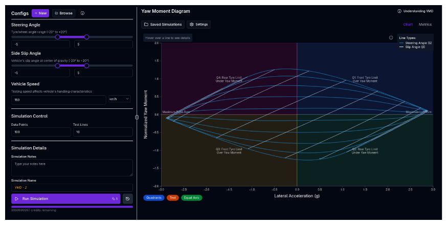
How to Read a YMD
The YMD plots Lateral Acceleration ($a_y/g$) on the X-axis and Yaw Moment Coefficient ($C_N$) on the Y-axis.
The Key Components
-
Constant Steering Lines ($delta$ curves):
- These lines represent holding the steering wheel fixed while the car slides at different angles.
- Slope = Stability.
- Negative Slope (): Stable. If the car gets disturbed (yaw moment increases), it naturally generates a restoring moment to straighten out.
- Positive Slope (/): Unstable. A disturbance amplifies itself, leading to a spin.
- Crossing X-axis ($C_N=0$): This is the steady-state "trim" point where the car holds a constant radius.
-
Constant Sideslip Lines ($beta$ curves):
- These lines represent maintaining a constant drift angle while changing steering.
- The vertical spacing between these lines indicates Control Power (how much yaw moment you get per degree of steering).
-
The Envelope:
- The outer boundary of the "carpet plot" represents the physical limits of the vehicle's tyre grip and aerodynamics.
Handling Metrics
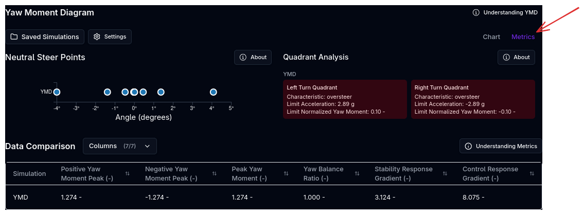
The Handling Metrics panel shows at limit metrics, such as oversteer/ understeer, limit acceleration and yaw moment, and the Limit Points of the YMD.
Simulation Settings
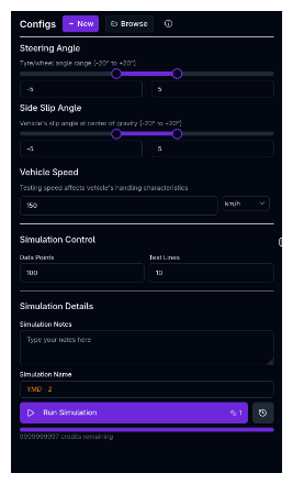
1. Ranges
You define the boundaries of the "state space" you want to explore: - Steering Angle ($delta$): Range of front wheel angles (e.g., -5° to +5°). - Side Slip Angle ($beta$): Range of vehicle drift angles (e.g., -5° to +5°).
2. Vehicle Conditions
Speed: The simulation runs at a constant velocity. - Low Speed (e.g., 60 km/h): Dominant mechanical handling (springs, ARBs, mechanical trail). - High Speed (e.g., 200 km/h): Dominant aerodynamic handling (CoP position, aero mapping).
Longitudinal Acceleration: Optionally apply a constant longitudinal acceleration to study combined braking or traction conditions. - Negative values (down to −5 g): Braking — simulates trail braking into a corner. - Positive values (up to +1 g): Traction — simulates power application at corner exit. - 0 g (default): Pure lateral analysis (existing behaviour). - Accepts all standard acceleration units (g, m/s², ft/s²).
Combined Loading
Under trail braking or traction, longitudinal load transfer shifts the YMD balance significantly. Running the simulation at two or three longitudinal acceleration values alongside different speeds gives a complete picture of the combined-slip operating envelope.
3. Advanced Kinematics
An Advanced Kinematics toggle is available in the simulation settings (enabled by default). When on, the solver uses the full kinematics model — including ARB motion ratio curves, non-linear camber, toe, and roll centre geometry from your Kinematics setup — rather than simplified constant-value representations. The setting persists with the simulation configuration.
4. Resolution
- Test Lines: How many constant-$delta$ and constant-$beta$ curves to plot.
- Data Points: How many points to calculate along each line. Higher values give smoother curves but take longer to compute.
Computational Cost
The total number of equilibrium solves is 2 x Test Lines x Data Points (one set of sweeps for constant-$delta$ lines, another for constant-$beta$ lines). For example, 10 test lines with 50 data points produces 1,000 solves. Start with moderate resolution (e.g., 8 lines, 30 points) and increase if you need smoother curves.
Running a Handling Simulation
- Ensure your vehicle setup is complete (chassis, suspension, aerodynamics, tyres at minimum)
- Navigate to the Handling simulation page
- Set the Steering Angle and Side Slip Angle ranges
- Set the Speed for the analysis
- Optionally set a Longitudinal Acceleration for combined braking/traction studies
- Configure Resolution (Test Lines and Data Points)
- Enter a Simulation Name and optional notes
- Click Run Simulation
Choose a Relevant Speed
Pick a speed representative of the corner you are analysing. Use a low speed (e.g., 60 km/h) for slow hairpin balance, or a high speed (e.g., 200 km/h) for fast-corner aero stability. Running at two or three speeds gives a complete picture of how balance shifts with aero load.
Physics Engine
The Handling simulation uses the same high-fidelity Lateral Convergence solver as the Cornering simulation. For every point on the grid ($delta, beta, v$), it solves the full static equilibrium of the vehicle, accounting for:
- Tyre Nonlinearity: Combined slip, load sensitivity, and camber thrust.
- Suspension Kinematics: Bump steer, roll steer, and camber change.
- Aerodynamics: Ride height sensitivity and aero balance shifts.
- Load Transfer: Elastic, geometric, and unsprung weight transfer.
Warm Starting
To ensure speed and robustness, the solver uses "warm starting," using the solution from the previous grid point as the initial guess for the next. This allows generating thousands of equilibrium points in seconds.
Tips & Best Practices
Analyzing Roll Stiffness Distribution
The slope of the constant steering lines is heavily influenced by the distribution of roll stiffness (Springs + ARBs). - Stiffening the Front: Shifts balance towards understeer (lines slope more negatively). - Stiffening the Rear: Shifts balance towards oversteer (lines flatten or slope positively).
See our GT3 Case Study for a practical example.
Aero Stability
Run the simulation at high speed (e.g., 200 km/h) to check aerodynamic stability. If the constant steering lines slope upwards (positive slope) at high g, the car is aerodynamically unstable—the center of pressure might be moving forward as ride heights change in the corner, leading to a high-speed spin risk.
The Limit
Look at the maximum X-value (Lateral G). - If the plot "closes off" on the right (lines converge), the car is limit stable (understeer limit). - If the lines flare open or hook upwards at the limit, the car is limit unstable (snap oversteer risk).
Related Topics
- Cornering Simulation — Finds the specific limit points along the $C_N=0$ axis.
- Suspension Setup — Adjust ARBs and springs to tune the YMD shape.
- Aerodynamics — Adjust Aero Balance to change high-speed stability.