Track Configuration

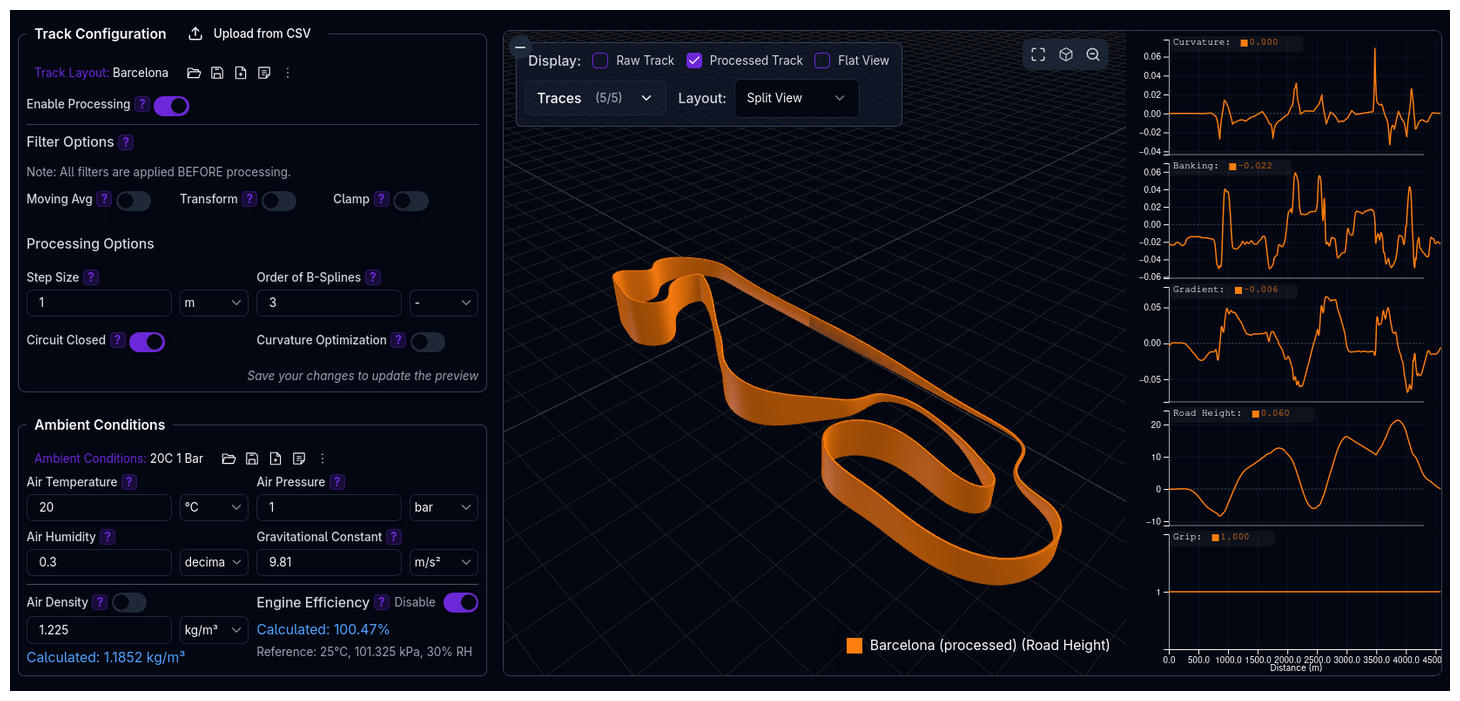
Configure the track for your lap time simulations. Build a track from satellite imagery or upload logged data, apply processing, optimise a racing line, and visualise the result.

Overview

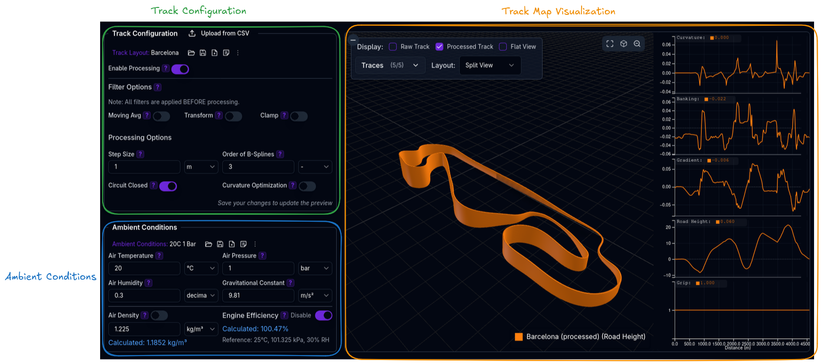
The Track page is split into two columns:

• Left column — Track configuration (library, upload, filters, processing), the Racing Line panel, and Ambient Conditions
• Right column — Track map visualization and trace charts

Two buttons sit above the setup palette:

Button	Purpose
New track	Start a track from scratch, drawn directly on satellite imagery.
Edit current track	Open the Satellite Track Editor for the loaded track.

---

Track Configuration

The track configuration section uses the standard Setup Command Palette for saving, loading, and duplicating track setups from your library.

---

Standard and Legacy Processing

Tracks exist in one of two processing modes.

Standard is the current pipeline. Track geometry is defined by its boundaries — the outer and inner tarmac edges — from which the centreline and width profile are derived. Smoothing is reduced to a single strength choice.

Legacy is the original pipeline, where geometry is a centreline plus manually tuned filter knobs. Legacy tracks show a deprecation banner with a Convert action.

Legacy tracks can no longer run simulations

Legacy support ended on 2026-08-14. A track still in legacy mode is blocked from launching new simulations until it is converted, and the banner on the Track page links straight to the conversion. Opening a legacy track with no width data now opens the width conversion dialog automatically. Converting does not affect your stored simulation results.

The Filter Options and Processing Options sections below document the legacy knobs, which remain visible in legacy mode. In standard mode, smoothing collapses to:

Preset	Behaviour
Off	No smoothing applied.
Light	Savitzky-Golay, 11-point window, cubic.
Strong	Savitzky-Golay, 31-point window, cubic.

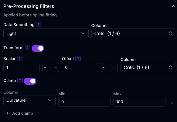
The preset sets smoothing strength only. Which columns are smoothed stays your choice — Curvature is seeded as the default when nothing is selected. Transform and Clamp remain available in both modes.

Track width is also standard-mode only: where a track has no width columns, a single Track width value is used as the fallback. A track carrying width columns from its source file says so instead.

---

Satellite Track Editor

The satellite editor is where track geometry is created and changed. It overlays the track on satellite imagery so the boundaries can be matched to the real tarmac.

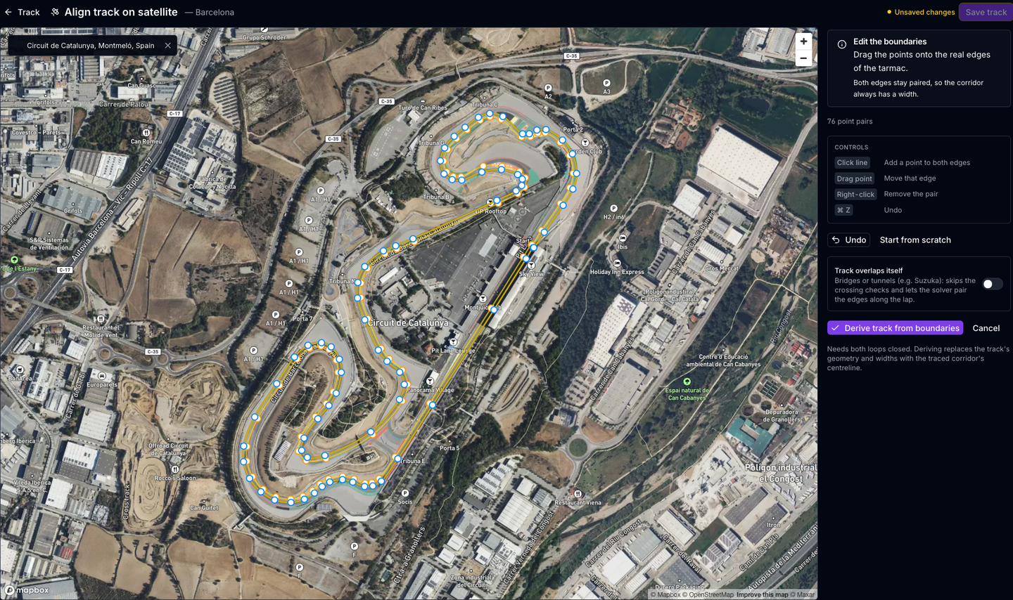
Open it with Edit current track, or New track to draw one from nothing.

Placing the track

An unplaced track floats above the map until it is anchored:

• Adjust placement — move, rotate and rescale the track over the imagery.
• Center on track — recentre the viewport.

Once placed, the track is anchored to real-world coordinates and you can pan and zoom freely.

Editing boundaries

Edit boundaries is the primary way to change track geometry — the boundaries define the track.

Both edges are always paired: every point on one edge has a partner on the other, so the corridor always has a width. Editing gestures:

Gesture	Action
Click line	Add a point to both edges
Drag point	Move that edge
Right-click	Remove the pair
Click first point	Close the loop
⌘/Ctrl-Z	Undo

When drawing a new track, you are first asked to place the start/finish line — click one edge of the tarmac where the lap starts, then click straight across on the opposite edge. That single gesture sets both the start line and the initial track width. From there, trace along one edge and the opposite edge follows automatically at the learned width.

While tracing, a control above the map lets you declare whether you are drawing the outer or the inner edge, rather than leaving it to be inferred once the loop closes. The edge you are actively adding points to is highlighted in blue and the edge following automatically in amber, so it is always clear which line your next click lands on. Once the loop is closed, the panel states plainly which edge is leading and which is following.

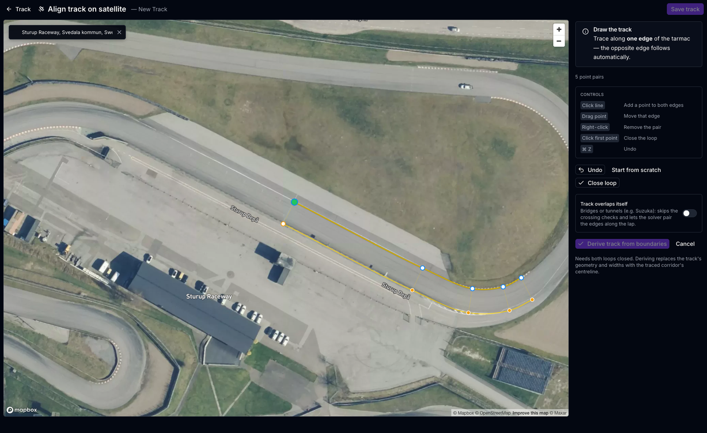
The point counter reads point pairs, not points — a reminder that the two edges move together. Close loop becomes available once at least three pairs exist.

Derive track from boundaries replaces the track's geometry and widths with the traced corridor's centreline. Both loops must be closed first.

Tracks that cross themselves

Enable Track overlaps itself for circuits with bridges or tunnels (Suzuka, for example). This skips the crossing checks and lets the solver pair the edges along the lap.

Rebuilt boundaries

Your traced boundaries are saved with the track. If the geometry later changes — a re-upload, a moved start line — the trace no longer matches, and the editor shows edges rebuilt from the centreline and width instead. You will see a notice saying so. A rebuilt edge cannot reproduce a corner tighter than the half-width, so it will not match what you originally drew. Adjust and derive again to replace it.

Other editor actions

Action	Description
Move start line	Click anywhere on the circuit to snap the Start tick to the nearest point, or drag the tick along the lap. Applying rotates the lap so Distance 0 starts there. Sectors keep their physical position.
Flip driving direction	Reverses the order of all track points. Start/finish stays at the same physical position.
Sample road heights from terrain	Fills the elevation profile from satellite terrain data (~10–30 m resolution). Gradient is recomputed on save; banking is unaffected.

Recompute the racing line

Moving the start line or flipping direction changes the geometry — recompute the racing line afterwards.

---

Local grip

The Local grip section of the editor sidebar lets you mark individual stretches of the lap as damp, dusty, worn or unusually grippy, without altering the tyre model or the whole-session grip figure.

Creating zones

Action	Description
Click the track	With the section open, clicking anywhere on the circuit drops a zone at that point.
Add	Creates several placeholder zones at once, to be positioned afterwards.
Clear all	Removes every zone from the track.

Each zone has three values:

Field	Description
Start	Distance around the lap where the zone begins.
End	Distance around the lap where the zone ends.
Factor	Grip multiplier. 1.0 leaves grip unchanged, below 1.0 reduces it, above 1.0 raises it. Must be greater than zero.
Blend	Distance over which the factor eases in and out at each edge, instead of switching on and off abruptly.

Zones may overlap deliberately. Where they do, whichever zone you added or moved most recently takes precedence over that stretch, and the table flags the earlier zones it is sitting on top of.

Reading the map

• Grip is drawn as a red-to-blue band over the satellite imagery — red for raised grip, blue for reduced, white for neutral — with the numeric endpoints of the colour scale shown beside the legend. The scale is fitted per track.
• Selecting a zone in the list highlights that stretch with a yellow halo and exposes S and E drag handles on the map for adjusting where it starts and ends.
• A coverage indicator reports what percentage of the lap currently carries a zone.
• A toggle controls whether the grip colouring stays visible once the Local grip section is closed. While you are actively editing, it is always shown.

Local zones replace an uploaded grip map

If the track already carries a measured grip map from an upload or survey, adding zones here replaces it — the editor warns you before this happens. You can also upload a measured grip map from this same panel instead of drawing zones by hand.

Three factors multiply at the tyre

Grip at the contact patch is the product of the tyre model itself, any local zone covering that point, and the whole-session Track Grip value in Ambient Conditions. A 90% ambient grip over a local zone of 0.8 gives an effective 0.72 on that stretch.

---

Racing Line

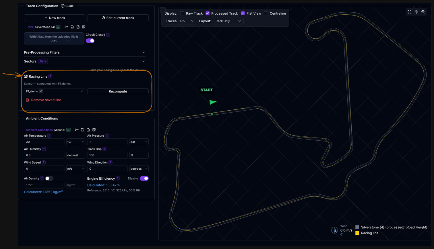
The Racing Line panel optimises the driven trajectory within the track corridor for a chosen vehicle and saves it to the track. Simulations then run on the saved line, which is fast and keeps lap times comparable across setups.

The saved line is drawn on the track map alongside the centreline, so you can see where it differs.

Pick a vehicle, then Compute racing line. The computed lap time is shown, and you can Save to track or Discard. A saved line can be removed with Remove saved line.

Requires width data

The panel is disabled without track width data — the optimiser needs a corridor to work within.

A Stale badge appears when the track geometry has changed since the line was computed. Recompute to bring it up to date.

Without a computed racing line, simulations drive the middle of the corridor.

---

Creating and Uploading a Track

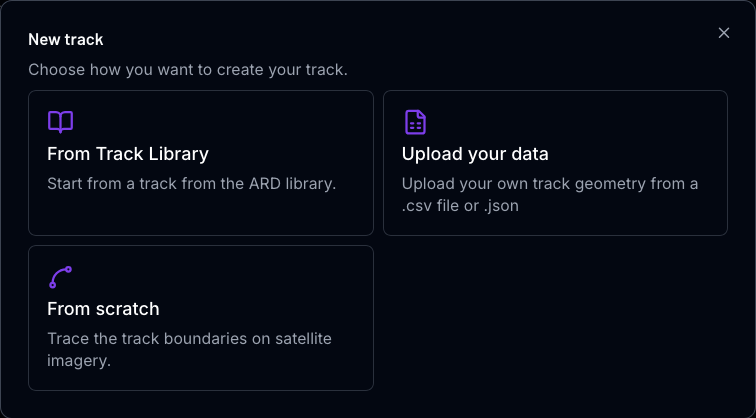
Click New track to choose how the track is created.

Option	Description
From Track Library	Start from a track in the ARD library.
Upload your data	Upload your own track geometry from a .csv or .json file.
From scratch	Trace the track boundaries on satellite imagery — opens the Satellite Track Editor.
Import ARD file	Re-import a track previously exported from ARD as JSON. The export already carries the geometry and georeferencing, so there is no mapping step.

Have a full telemetry export instead of a plain geometry file?

Upload your data here expects a track-geometry file — just the columns described in Track Data Columns below (or a VBox file), with no extra channels. A logger export with dozens of channels (PiToolbox, AiM, MoTeC, etc.) will not parse correctly here.

For that kind of file, upload it as telemetry instead: go to Results → Upload Telemetry, map its channels, and use the Create Track from Telemetry option on the final step. See Results Upload — Track Creation for the channel combinations that enable it.

The upload wizard

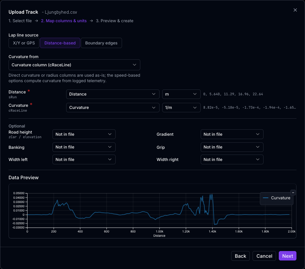
Upload runs as a series of steps:

Step	Purpose
Select file	Choose or drop the file. The format is detected automatically from our list of supported formats. CSV must not include a unit row
Map columns & units	Match each column in your file to a track quantity and set its units.
Options	Resolve conflicts and confirm GPS handling.
Preview & create	Review the parsed track on a map before creating it.

Not every step appears for every file. The Options step is shown only when there is something to resolve — a conflict, or a GPS notice. Track outline JSON skips column mapping, and VBox files go straight from selection to preview.

You cannot leave Map columns & units while two columns are mapped to the same quantity, or while the track has no usable line definition.

Lap line source

Choose how the track's line is defined:

Source	Requires
X/Y or GPS	X/Y coordinate columns, or latitude/longitude.
Distance-based	A distance channel plus a curvature source (below).
Boundary edges	Left and right boundary columns.

Curvature from

When the line is distance-based, curvature can come from four sources:

Source	Columns used
Curvature column	Curvature
Corner radius	Corner Radius
Speed + lateral acceleration	Speed, Lateral Acceleration
Speed + yaw rate	Speed, Yaw Rate

Direct curvature and radius columns are used as-is. The speed-based options compute curvature from logged telemetry, which is useful when your logger recorded vehicle motion but no geometry channel.

Each mapped column shows a preview of its first few values, and a Data Preview chart plots the selected channel so you can spot a wrong unit or a mis-mapped column before creating the track.

Road height, gradient, banking, grip and left/right width are optional — leave them as Not in file if your data does not carry them.

Multi-lap data

Logged telemetry often contains several laps. The wizard detects lap boundaries automatically — from a distance channel where one exists, otherwise by tracking how far the path winds around the track's own centroid — and lets you pick which lap to use.

Partial final laps

A trailing fragment covering less than a quarter of a turn is treated as the end of the data rather than a further lap, so the tail of a single lap is not split off as a phantom extra one.

CSV Format

The CSV file must use comma-separated values with column headers in the first row. Do not include units in the headers.

Example headers:

Distance,Curvature,X_cord,Y_cord,Banking,Gradient,Road Height,Grip

An example CSV file is available for download from within the upload dialog.

Track Data Columns

Column	Unit	Required	Description
Distance	m	Conditional	Cumulative distance along the track centerline. Required if X/Y coordinates are not provided.
Curvature	1/m	Conditional	Track curvature at each point. Positive = left turn. Required if X/Y coordinates are not provided.
X_cord	m	Conditional	X coordinate of the track centerline. Required if Distance/Curvature are not provided.
Y_cord	m	Conditional	Y coordinate of the track centerline. Required if Distance/Curvature are not provided.
Banking	rad	Optional	Track banking angle. Defaults to 0.
Gradient	rad	Optional	Track gradient (slope) angle. Defaults to 0. Auto-calculated from Road Height if provided.
Road Height	m	Optional	Elevation of the track surface. Used to derive Gradient if Gradient is not supplied.
Grip	0–1	Optional	Surface grip multiplier. Defaults to 1.
Width_left	m	Optional	Half-width of the track corridor to the left of the centerline at each point.
Width_right	m	Optional	Half-width of the track corridor to the right of the centerline at each point.

What Width_left/Width_right are for

Supplying per-point Width_left/Width_right gives the track a real corridor to work within, instead of falling back to a single uniform Track width value. This corridor is what the Racing Line optimiser stays inside of, and it also bounds how far a simulation is allowed to deviate from the provided trajectory — without it, deviation defaults to a narrow tolerance around the centerline/racing line rather than the true track boundaries.

Coordinate Input Options

You can provide either Distance + Curvature or X/Y coordinates. If both are provided, X/Y coordinates take priority and Distance/Curvature are recalculated from them.

GPS Coordinates

GPS (latitude/longitude) coordinates are auto-detected and converted to local X/Y in meters. Place latitude values in X_cord and longitude values in Y_cord.

GPS values are range-checked

If you mark your X/Y columns as GPS degrees, the values are validated against the WGS84 range — latitude must fall between -90 and 90, longitude between -180 and 180. Values in meters (or eastings/northings) tagged as degrees, or latitude and longitude entered the wrong way round, are rejected at upload with a message naming the range that was breached.

While you are still on the column-mapping step, a These don't look like GPS degrees banner appears as soon as an out-of-range value is seen, naming the offending column. Previously a mismatched unit produced a track in a nonsensical location that could fail to open in the satellite editor.

---

Processing Pipeline

Track data flows through a two-stage pipeline: Filters are applied first, then Processing.

flowchart LR
    A[Raw CSV Data] --> B{Processing Enabled?}
    B -->|Yes| C[Filters]
    C --> D[Processing]
    D --> E[Final Track]
    B -->|No| E

A master toggle Enable Processing controls whether the pipeline runs. When disabled, the raw uploaded data is used directly in simulations.

---

Filter Options

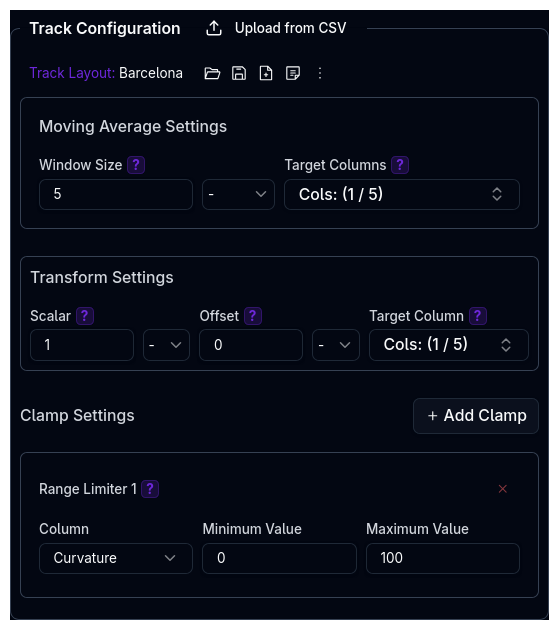
Legacy mode

The individual filter knobs below are exposed in legacy mode. In standard mode, smoothing is a single Off / Light / Strong choice — see Standard and Legacy Processing.

Filters are applied before spline processing. They clean and adjust the raw data.

Smoothing

Smooths noisy data before spline fitting. Two methods are available:

Savitzky-Golay (Recommended)

Fits a polynomial to each sliding window and evaluates it at the center point. Unlike a simple moving average, this preserves curvature peaks in chicanes and tight corners — the polynomial can represent the parabolic shape of a peak without attenuating it.

Parameter	Description
Window Length	Number of data points in the polynomial fit window. Must be odd. At 2m spacing, 11 covers ~22m of track.
Polynomial Order	Degree of the fitted polynomial. Order 3 (cubic) is recommended for most tracks. Must be less than window length.
Target Columns	Which columns to smooth: Curvature, Banking, Gradient, X & Y Coordinates.

When to Use Savitzky-Golay

Use this for GPS-logged or Formula Student data where preserving the shape of tight corners matters. A moving average with the same window size would flatten a hairpin by ~15%, while Savitzky-Golay preserves it within ~1%.

Moving Average (Legacy)

Smooths data by averaging over a sliding window. Simple but can flatten curvature peaks.

Parameter	Description
Window Size	Number of data points to average over. Larger values produce smoother results.
Target Columns	Which columns to smooth.

Transform

Applies a linear transformation (scale and offset) to selected columns.

Parameter	Description
Scalar	Multiplier applied to column values. Values of 0.95–1.05 are recommended for loop-closing adjustments.
Offset	Additive constant applied after scaling.
Target Columns	Which columns to transform.

Clamp

Limits column values to a specified range, removing outliers. You can add multiple clamp configurations, each targeting a different column.

Parameter	Description
Column	The data column to clamp.
Min Value	Lower bound — values below this are clamped.
Max Value	Upper bound — values above this are clamped.

Clamp for Curvature

Clamping curvature is useful for removing GPS spikes or sensor glitches that produce unrealistically sharp corners.

---

Processing Options

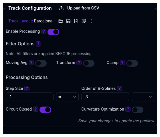
Legacy mode

Standard-mode tracks derive their geometry from traced boundaries in the Satellite Track Editor, so most of these knobs are not surfaced. They remain available on legacy tracks.

Processing options are applied after filters. They interpolate and standardize the track geometry.

Step Size (m)

The distance increment for interpolated track points. We recommend a step size of 1–3 m. A step size of 3 m is ideal for faster lap time computation, particularly on longer circuits (above ~4 km).

The step size should match or be coarser than the spacing in your supplied data. Setting it finer than your raw data resolution adds noise without improving accuracy.

Step Size and Simulation Granularity

A very coarse step size (e.g., 10 m) produces granular lap simulation results — the solver has fewer points to work with and corner entry/exit speeds become less accurate. Conversely, a very fine step size on a long circuit increases computation time significantly.

Validation: Step size must be ≥ 0.1 m.

Order of B-Splines

The polynomial degree used for spline approximation, from 1 (linear) to 5 (quintic).

Order	Description
1	Linear interpolation — no smoothing. Suitable for straight-line tracks only.
2	Quadratic — not recommended (even orders can produce artifacts with small smoothing).
3	Cubic — decent default. Good balance of smoothness and fidelity for most circuits.
4	Quartic — not recommended.
5	Quintic — highly recommended for larger circuits. Most accurately captures corners and chicanes, especially when combined with Curvature Optimization.

Choosing the Right Order

• Use order 1 only for straight tracks (constant-curvature or zero-curvature sections).
• Use order 3 as a starting point for general circuits.
• Use order 5 for longer or more complex circuits — it captures tight corner sequences and chicanes more faithfully than cubic splines.
• Odd-degree splines (3, 5) generally behave better than even degrees (2, 4), especially with small smoothing factors.

Spline Stiffness

Controls how aggressively the B-spline smooths the track geometry. When disabled (default), the stiffness is automatically calculated based on the number of track points. When enabled, you can manually set the value.

• Lower values (e.g., 5–50) preserve tight corners and chicanes but are more sensitive to noise.
• Higher values (e.g., 200+) produce smoother curves but may flatten sharp features.
• Auto (toggle off) scales with the track point count — works well for most cases but can over-smooth small circuits.

Formula Student Tracks

FS circuits are typically short (300–500m) with tight corners. The auto stiffness often over-smooths these. Try setting stiffness to 10–30 with the Savitzky-Golay pre-filter enabled for the best results.

Circuit Closed

When enabled, the track start and end points are smoothly connected to form a continuous loop. Disable this for non-circuit tracks (e.g., hillclimbs, point-to-point stages).

Circuit Closed also controls flying laps

This switch does more than smooth the join. An open circuit has no closed lap to carry speed round to the start line, so with Circuit Closed off the Lap Time simulation no longer offers Flying Lap — it shows a locked Off — open circuit badge instead, and the run starts from rest. Turn Circuit Closed on if the track really is a full lap.

How the Stretching Method Works

Real-world track data rarely closes perfectly — the last recorded point almost never lands exactly on the first. The closure algorithm corrects this gap without distorting the track shape.

The algorithm works in two phases:

1. Heading correction — It calculates the heading (direction of travel) at every point along the track. If there is a heading error between the start and end (i.e., the track doesn't point back the way it started), this error is distributed linearly along the entire track length. Each point's heading is adjusted by a small fraction of the total error, proportional to its distance along the track. The track coordinates are then reconstructed from these corrected headings.

2. Position correction — After heading correction, a small positional gap may remain between the reconstructed start and end points. This residual gap is removed by applying a linear spatial shift distributed along the track — points near the start are barely moved, while points near the end absorb most of the correction. The final point is then snapped exactly to the start position.

The result is a smoothly closed circuit where the correction is spread across the entire track rather than concentrated at the join point. This preserves the original track shape while ensuring the circuit forms a proper loop.

Already Closed Tracks

If the start and end points are already within 1 meter of each other, the algorithm skips closure — the track is considered already closed.

Curvature Optimization

Curvature optimization uses quadratic programming (QP) to produce a smoother curvature profile. This is particularly useful for GPS-sourced track data where sensor jitter introduces noise into the curvature.

How It Works

At each point along the processed track, the spline fitting step produces a normal vector — a direction perpendicular to the track centerline. The optimizer is allowed to shift each point laterally along its normal vector (left or right) by a bounded amount, constrained by the track width so that the shifted point remains within the track boundaries.

The optimizer solves a QP problem to find the set of lateral shifts that minimizes curvature variation across all points simultaneously. It uses a curvature_matching objective by default, which penalizes deviations in the shift profile's second derivative relative to the reference curvature — effectively smoothing out noise while preserving the genuine shape of corners.

The key constraints are:

• Track boundaries — Each point's lateral shift is bounded by the track width (minus half the vehicle width as a safety margin). Points cannot be moved outside the track edges.
• Continuity — The QP formulation uses finite-difference approximations of second derivatives, ensuring the resulting path remains smooth rather than producing abrupt jumps.

The result is a track centerline with a cleaner curvature profile that still faithfully follows the physical track layout. Genuine corners are preserved; GPS noise and small jitters are removed.

When to Use Curvature Optimization

Enable this when your track data comes from GPS logging or other noisy sources. It pairs well with order 5 B-splines for the best results on complex circuits. For clean, hand-measured or CAD-sourced track data, optimization is usually unnecessary.

---

Curvature Quality and Lap Time Accuracy

Curvature Directly Drives Lap Time Results

The curvature profile is the single most important input to the QSS lap time simulation. The solver uses curvature at every point to determine the maximum cornering speed — noisy or inaccurate curvature leads to unrealistic speed traces and incorrect lap times.

Spend time making the curvature profile smooth and realistic before running simulations. Use the trace charts to inspect the curvature channel visually. Look for:

• Spikes or oscillations — signs of GPS noise or insufficient smoothing. Apply moving average filters, increase B-spline order, or enable curvature optimization.
• Flat curvature in corners — the spline may be over-smoothing. Reduce the step size or use a higher-order spline to capture the corner shape.
• Discontinuities at the start/finish — enable Circuit Closed to eliminate the join artifact.

A smooth, accurate curvature profile is the foundation of realistic lap time simulation results.

---

Sectors

Sectors divide the track into segments for per-sector analysis — sector times, speeds, g-forces, and energy usage are computed for each sector independently.

Automatic Sectoring

By default, sectors are detected automatically from curvature sign changes (left turn → right turn transitions). This produces a reasonable breakdown but may not match official timing sectors.

Manual Sectors

Open the Sectors section in the track configuration to define your own sector boundaries by start and end distance (in metres). Use the "Add N sectors" input to quickly create multiple sectors.

• Toggle Sectors in the track map display controls to visualise sector boundaries with colour-coded segments.
• The coverage indicator warns if your sectors don't cover the full track length.
• Sectors are numbered automatically (S1, S2, S3...) and flow through to all per-sector metrics in simulation results.

Sectors and Metrics

Manual sectors override automatic detection. When defined, all simulation metrics (sector times, speeds, energy) use your sector boundaries. When empty, the automatic curvature-based sectors are used.

---

Tips and Troubleshooting

Noisy Data (Formula Student / GPS)

GPS-logged track data often contains noise that causes unrealistic speed profiles. Recommended approach:

1. Enable Savitzky-Golay smoothing under Pre-Processing Filters — preserves curvature peaks while removing noise.
2. Set a lower Spline Stiffness (5–50) — keeps the trajectory closer to your original data.
3. Increase B-Spline Order to 5 — produces smoother curvature transitions for the lap time simulation.

Smooth Speed Profiles in QSS

The QSS lap time simulation is very sensitive to curvature noise — small spikes create unrealistic acceleration jumps. Key controls:

• Spline Stiffness is the primary lever. Higher = smoother but may flatten chicanes.
• B-Spline Order 5 generally produces smoother curvature rate-of-change than order 3.
• Curvature Optimization shifts points laterally to reduce curvature variation while respecting track boundaries. Enable this if you see the processed track deviating from the original shape.

Loop Closure Distortion

If the closure algorithm distorts your track shape:

1. Use Transform — apply a small scalar (0.99–1.01) to X & Y coordinates to bring the start/end points closer together before the closure algorithm runs.
2. Check your source data — if the gap exceeds 5% of track length, consider trimming or extending your logged data.
3. Disable Circuit Closed for open-ended tracks (hillclimbs, drag strips).

Processing Pipeline Order

Understanding the order helps diagnose issues:

1. Pre-Processing Filters — Smoothing, Transform, Clamp applied to raw input
2. Coordinate Generation — if data is Distance + Curvature, X/Y are reconstructed
3. Loop Closure — start/end points joined (if Circuit Closed is on)
4. B-Spline Fitting — smooth curve fitted through points (Step Size, Spline Order, Spline Stiffness)
5. Curvature Optimization — optional QP smoothing (if enabled)
6. Sector Assignment — automatic or manual sector boundaries applied

Filter Interaction with Data Format

For Distance + Curvature tracks, smoothing the curvature column changes the reconstructed X/Y path — the filter has a real effect. For X/Y coordinate tracks, smoothing the curvature column has no effect because the B-spline re-derives curvature from the fitted curve. In this case, consider smoothing the X & Y columns directly.

Note that Distance itself is not a filterable column and is no longer offered in any of the filter column pickers. It is the abscissa the other channels are measured against, not a channel in its own right; selecting it used to make every attempt to process or simulate that track fail. Any existing track that had Distance selected has had it removed automatically — the rest of your filter configuration is untouched. If such a track had a saved racing line, it is flagged as out of date and should be recomputed.

---

Track Visualization

The right side of the Track page displays the track map and trace charts.

Display Toggles

Toggle	Description
Raw Track	Shows the unprocessed track data on the map.
Processed Track	Shows the filtered and processed track data.
Flat View	Removes elevation from the visualization. Only appears when the track has height data.
Sectors	Colour-codes the track by sector boundaries. Only appears when sectors are defined.

Layout Presets

Layout	Description
Split View	Track map and trace charts side by side.
Track Only	Full-screen track map.
Trace Only	Full-screen trace charts.

A Trace Selector lets you choose which data channels (curvature, banking, gradient, etc.) to display in the trace charts. Deselected channels are hidden, and rows with no visible channels are removed from the chart area.

---

Validation Notes

• Step size must be ≥ 0.1 m
• B-spline order must be between 1 and 5 (odd orders recommended)
• CSV must contain either Distance + Curvature or X/Y coordinates
• Grip values of 0 are automatically replaced with a small positive value (0.001)
• Local grip zone factors must be greater than zero
• Banking and Gradient values > 1 are assumed to be in degrees and auto-converted to radians

---

Related Topics

• Ambient Conditions — Air density, engine efficiency, wind speed, and whole-session track grip
• Aerodynamics Setup — Track-specific aero requirements
• Lap Time Simulation — Run simulations on your track
• Results — Analyze simulation output