Lap Time Simulation (QSS)
The Quasi-Steady-State (QSS) lap time simulation predicts how fast your vehicle can complete a circuit by solving the vehicle dynamics at every point around the track. It is the flagship simulation in ARD and the most comprehensive way to evaluate overall vehicle performance.
What is Quasi-Steady-State?
A quasi-steady-state simulation assumes that at each point along the track, the vehicle is in instantaneous equilibrium — all forces and moments balance as if the car were in a steady-state condition at that speed, curvature, and acceleration. The simulation then stitches these equilibrium solutions together to produce a continuous speed profile around the lap.
This is distinct from a fully transient (dynamic) simulation, which integrates the equations of motion forward in time. QSS trades some transient fidelity for dramatically faster solve times and robust convergence — making it the standard approach used across professional motorsport for setup optimisation and performance prediction.
QSS vs Dynamic Lap Time Simulation
ARD also offers a Dynamic Lap Time Simulation (currently in beta), which uses optimal control theory to solve the full transient equations of motion. The dynamic approach captures effects like weight transfer settling, tyre thermal transients, and driver behaviour that QSS cannot. However, it is significantly more computationally expensive and requires more careful parameterisation.
For the vast majority of vehicle setup work, QSS provides the right balance of accuracy, speed, and robustness.
How Racing Teams Use It
QSS lap time simulation is the workhorse of motorsport vehicle dynamics departments. Typical uses include:
- Setup optimisation — Evaluating the lap time impact of changes to springs, ride heights, aero balance, gear ratios, and differential settings
- Circuit preparation — Predicting performance at a new circuit before the car arrives, helping engineers arrive with a sensible baseline setup
- Aero configuration selection — Choosing between high-downforce and low-drag aero packages based on predicted lap time
- Tyre strategy — Understanding how tyre compound and degradation affect lap performance
- Regulation impact analysis — Quantifying the effect of regulation changes on performance (e.g., weight increases, aero restrictions)
- Development direction — Prioritising which areas of the car to develop by understanding sensitivity to different parameters
Strengths and Limitations
Strengths
- Fast solve times — A full lap completes in seconds, enabling rapid iteration and parameter sweeps
- Robust convergence — The solver converges reliably across a wide range of vehicle and track configurations
- Full vehicle model — Accounts for aerodynamics (with ride height sensitivity), suspension, powertrain, brakes, tyres, and track features (banking, gradient, grip)
- Energy management — For electric and hybrid vehicles, tracks battery state-of-charge, regenerative braking, and power limits across the lap
Limitations
- No transient effects — Cannot capture weight transfer settling, tyre thermal dynamics, or driver reaction times
- Assumes perfect driver — The solver finds the theoretical maximum performance at every point; real lap times will always be slower
- Single racing line — The simulation follows the provided track centreline and cannot optimise the racing line
- No tyre degradation — Performance is assumed constant throughout the lap (though multiple laps can be simulated with energy depletion for EVs)
- Simplified tyre-level outputs — The QSS approach uses a pre-computed performance envelope (the GGV diagram) to determine acceleration limits at each track point, rather than solving individual tyre forces in real time. This means the simulation does not produce individual tyre lateral forces, slip angles, or slip ratios. Longitudinal tyre forces are simplified. For detailed tyre-level analysis, use the Cornering Simulation or the Dynamic Lap Time Simulation (beta)
How the Simulation Works
The QSS solver runs in three sequential phases, each building on the previous one to progressively constrain the speed profile.
flowchart TD
    A[Phase 1: Maximum Cornering Speed] --> B[Phase 2: Braking Envelope]
    B --> C[Phase 3: Acceleration + Full Dynamics]
    C --> D{Flying Lap?}
    D -->|Yes| E[Re-run Phase 3 with converged start speed]
    D -->|No| F[Standing start]
    E --> G[Post-Processing & Metrics]
    F --> G
Phase 1 — Maximum Cornering Speed
The first phase establishes the upper speed limit at every point around the track. At each track point, the solver determines the fastest the car can travel through the given curvature while staying within the tyre grip envelope.
This is determined by the GGV diagram (see below). For each curvature value, the solver finds the highest speed at which the required lateral acceleration does not exceed the vehicle's lateral capability. Track grip multipliers and banking forces are accounted for.
The result is a speed profile that represents the pure cornering limit — the car could sustain this speed if it never needed to accelerate or brake.
Phase 2 — Braking Envelope (Backward Pass)
The second phase works backwards around the track, applying combined cornering and braking constraints. Starting from each corner apex (local speed minimum from Phase 1), the solver propagates backwards to determine how late the car can brake while respecting:
- The combined lateral and longitudinal grip envelope (friction ellipse from the GGV)
- Slope resistance forces
- The braking capability at the current speed
The result clips the Phase 1 profile to account for braking zones — the car must slow down before corners.
Phase 3 — Forward Integration (Full Dynamics)
The final phase integrates forwards around the track, applying the complete vehicle model:
- Powertrain — Gear selection, torque output, shift timing, efficiency losses
- Aerodynamics — Drag and downforce with ride height sensitivity, converged with the suspension model
- Suspension — Ride height changes under aero load and load transfer
- Braking — Mechanical brakes, engine braking (ICE), and regenerative braking (EV/hybrid), all distributed by brake bias
- Energy — Battery state-of-charge tracking, charge power limits, and regen recovery (EV/hybrid only)
At each point, the solver calculates the maximum acceleration the powertrain can deliver within the grip envelope, then takes the minimum of this and the Phase 2 braking profile. This produces the final, fully constrained speed profile.
For a flying lap, Phase 3 runs twice: the first pass establishes a baseline, and the second pass uses the end speed from the first pass as the starting speed, ensuring a self-consistent flying lap solution.
The GGV Diagram
The GGV (g-g-Velocity) diagram is the foundation of the QSS solver. It pre-computes the vehicle's acceleration limits across a range of speeds before the lap simulation begins. The GGV captures the relationship between:
- Lateral acceleration — How hard the car can corner
- Longitudinal acceleration — How hard the car can accelerate or brake
- Speed — How these limits change with velocity (due to aero, powertrain, and tyre load sensitivity)
What the GGV Contains
At each speed, the GGV stores four limit values:
- Maximum lateral acceleration — The peak cornering capability (e.g., turning right)
- Minimum lateral acceleration — The peak cornering capability in the opposite direction (e.g., turning left)
- Maximum longitudinal acceleration — The peak traction-limited acceleration
- Minimum longitudinal acceleration — The peak braking deceleration (including brake hardware limits and regenerative braking)
At any given speed, the combined lateral and longitudinal capability is modelled as a friction ellipse connecting these four limit points. This means that at full lateral acceleration, no longitudinal acceleration is available, and vice versa — with a smooth trade-off between them that matches real tyre behaviour.
How the GGV Captures Vehicle Performance
The lateral limits account for the full coupled vehicle state: tyre forces, suspension kinematics, roll, load transfer, aerodynamic downforce, and ride height effects. The longitudinal limits account for driven-wheel traction, brake hardware torque limits, engine braking, regenerative braking, and aero drag. All limits include load transfer convergence so that the tyre loads are self-consistent with the acceleration being produced.
Because the GGV is pre-computed, the lap simulation itself can evaluate performance at any (speed, curvature) combination very efficiently — it simply interpolates the pre-built tables rather than re-solving the full vehicle equilibrium at every track point.
GGV and Tyre-Level Detail
The GGV stores the vehicle's aggregate acceleration capability, not the individual tyre states that produced it. This is why the QSS lap simulation does not output individual tyre slip angles, lateral forces, or slip ratios — those quantities are solved during GGV construction but only the envelope limits are retained. If you need tyre-level detail, the Cornering Simulation provides this information at each speed point.
Simulation Settings
Flying Lap vs Standing Start
| Setting | Description |
|---|---|
| Flying lap | The car is already at speed when crossing the start/finish line. The solver iterates to find a self-consistent start speed. This is the standard mode for most circuit analysis. |
| Standing start | The car starts from rest. Useful for evaluating launch performance or race start scenarios. |
Lap Count
For electric and hybrid vehicles, running multiple laps tracks battery energy depletion across the stint. Each additional lap continues from the energy state at the end of the previous lap.
Advanced Kinematics
An Advanced Kinematics toggle is available (enabled by default). When on, the solver uses the full kinematics model — including ARB motion ratio curves, non-linear camber, toe, and roll centre geometry from your Kinematics setup — rather than simplified constant-value representations.
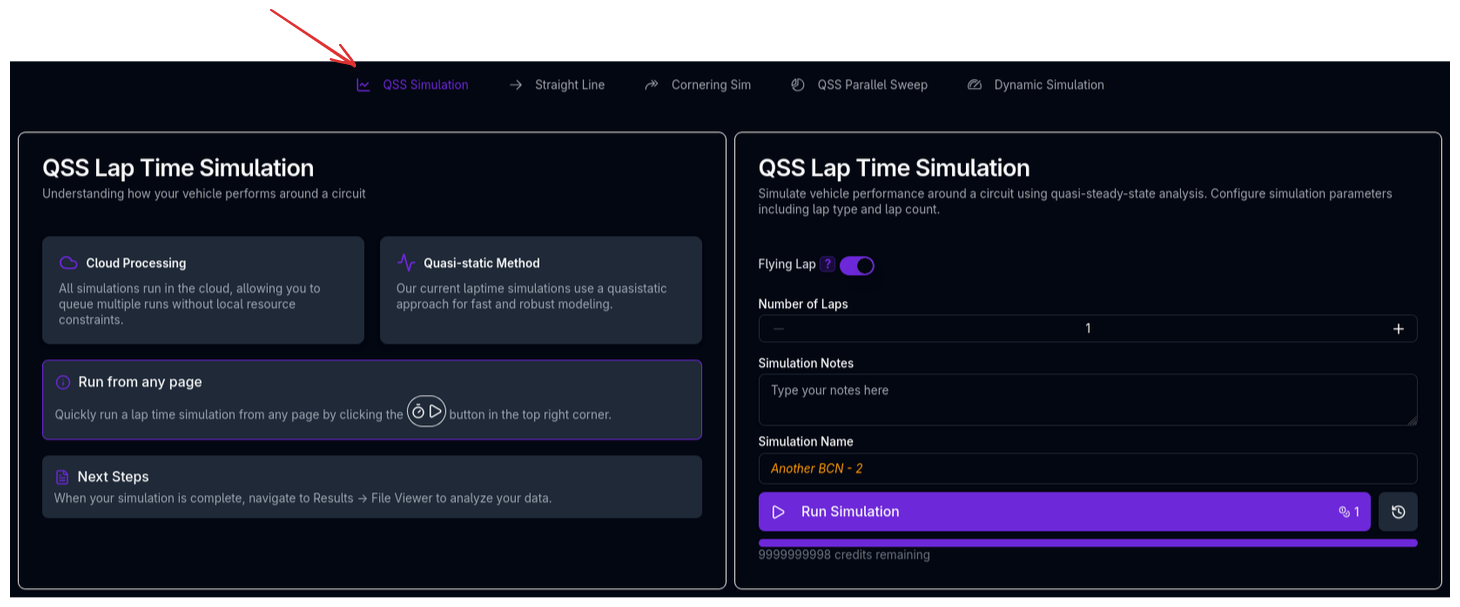
Running a QSS Lap Time Simulation
- Ensure your vehicle setup is complete (chassis, suspension, aero, powertrain, tyres, brakes)
- Ensure a track is loaded and processed (see Track Configuration)
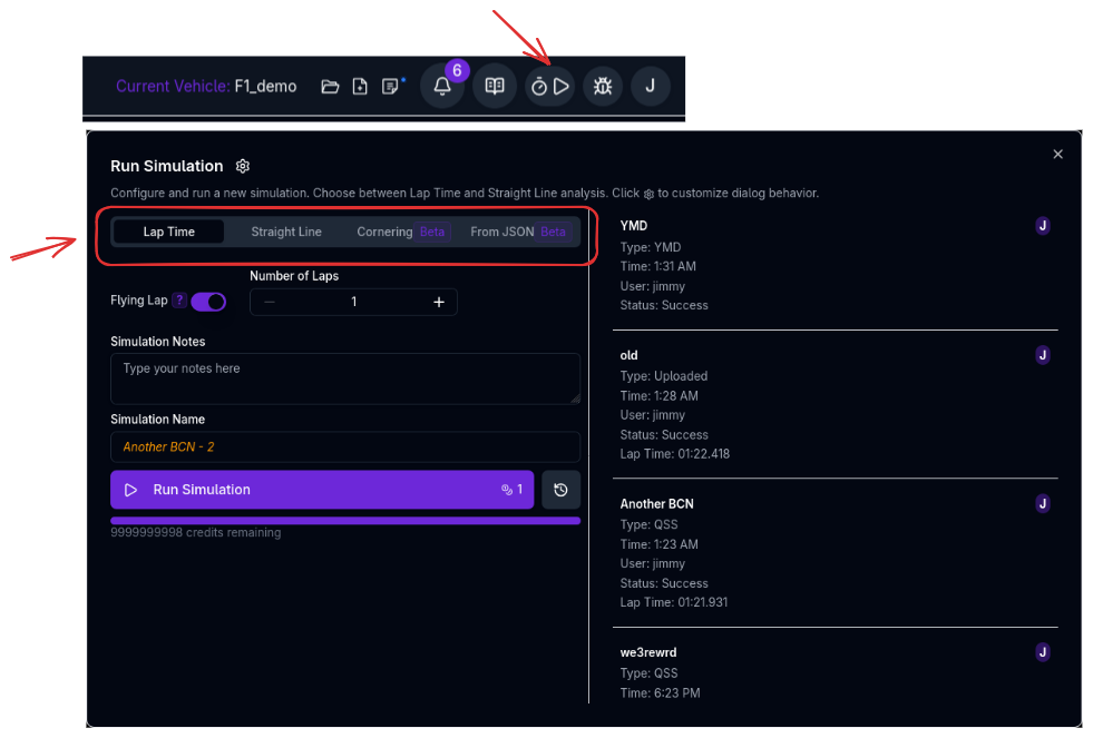
- Navigate to the Lap Time simulation page, or click the stopwatch icon in the navigation bar from any page
- Select Flying Lap or Standing Start
- Set the Lap Count (relevant for EV/hybrid energy tracking)
- Enter a Simulation Name and optional notes
- Click Run Simulation
Run from Any Page
You can launch a lap time simulation from any page in the application by clicking the stopwatch button in the top navigation bar. This opens a quick-run dialog without navigating away from your current work.
Key Outputs
The simulation produces a rich dataset at every track point. Key channels include:
| Channel | Description |
|---|---|
| vCar | Vehicle speed |
| gLat, gLong | Lateral and longitudinal acceleration |
| tRun, tDelta | Cumulative time and time per segment |
| FDrag, FLift | Aerodynamic forces |
| rAeroBal | Aerodynamic balance (centre of pressure) |
| CDrag, CLift | Aerodynamic coefficients (SCx, SCz) |
| hRideF, hRideR | Front and rear ride heights under aero load |
| xSuspF, xSuspR | Front and rear suspension displacement |
| FzFL, FzFR, FzRL, FzRR | Dynamic tyre loads at each corner |
| NGear, nEngine | Selected gear and engine/motor RPM |
| MPowertrain | Powertrain output torque |
| PPowertrain | Powertrain output power |
| MBrake, MBrakeF, MBrakeR | Brake torques (total, front, rear) |
| rBrakeBal | Effective brake balance |
| FResistanceTotal | Total resistance force (drag + slope + engine braking) |
| rSoc, ECapacity, VBattery | State of charge, remaining energy, and battery voltage (EV/hybrid) |
| nYaw | Yaw rate |
| aSteerNeutral | Neutral steer angle (geometric, from curvature and wheelbase) |
What the QSS Does Not Output
Because the QSS solver uses a pre-computed performance envelope (GGV) rather than solving individual tyre equilibria at each track point, the following quantities are not available from the lap time simulation:
- Individual tyre lateral forces (FyFL, FyFR, FyRL, FyRR)
- Tyre slip angles (aSlipTyreFL..RR)
- Tyre slip ratios (rSlipTyreFL..RR)
- Vehicle sideslip angle (set to zero)
- True steering angle (only the neutral steer angle is computed)
- Yaw moment from tyre forces
These quantities require solving the full tyre equilibrium at each point, which is what the Cornering Simulation and the Dynamic Lap Time Simulation (beta) provide. If you need to understand understeer behaviour, slip angle limits, or yaw moment balance around the lap, consider pairing your lap time results with a cornering simulation.
Tips & Best Practices
Start with Track Quality
The curvature profile is the single most important input. A noisy or inaccurate track will produce unreliable lap times regardless of how well the vehicle is modelled. See Track Configuration for guidance on processing track data.
Use for Relative Comparisons
QSS lap times are theoretical minimums that assume a perfect driver. They are most valuable for comparing configurations (e.g., "does this spring change improve or worsen lap time?") rather than predicting absolute lap times.
Pair with Cornering and Straight Line Simulations
If the lap time changes but you're not sure why, run Cornering and Straight Line simulations to isolate whether the gain comes from cornering performance, straight-line speed, or a balance change. The cornering simulation also provides the tyre-level detail that the QSS does not.
Check Your Vehicle Warnings
Before running a lap time simulation, review any vehicle validation warnings. Missing or inconsistent parameters (e.g., unrealistic tyre data, missing brake torque limits) can cause the solver to produce misleading results or fail to converge.
Related Topics
- Track Configuration — Prepare and process track data for simulation
- Cornering Simulation — Analyse steady-state cornering capability with full tyre-level detail
- Straight Line Simulation — Analyse aerodynamic and ride height behaviour at speed
- Trace View — Visualise and analyse simulation results
- Metrics — Review summary performance metrics